Coefficients.
Data Types | |
| type | coef_t |
| Coefficients defined on a given (mesh, \( X_h \)) tuple. Arrays use indices (i,j,k,e): element e, local coordinate (i,j,k). More... | |
Functions/Subroutines | |
| subroutine | coef_init_empty (this, xh, msh) |
| Initialize empty coefs for a space and a mesh. | |
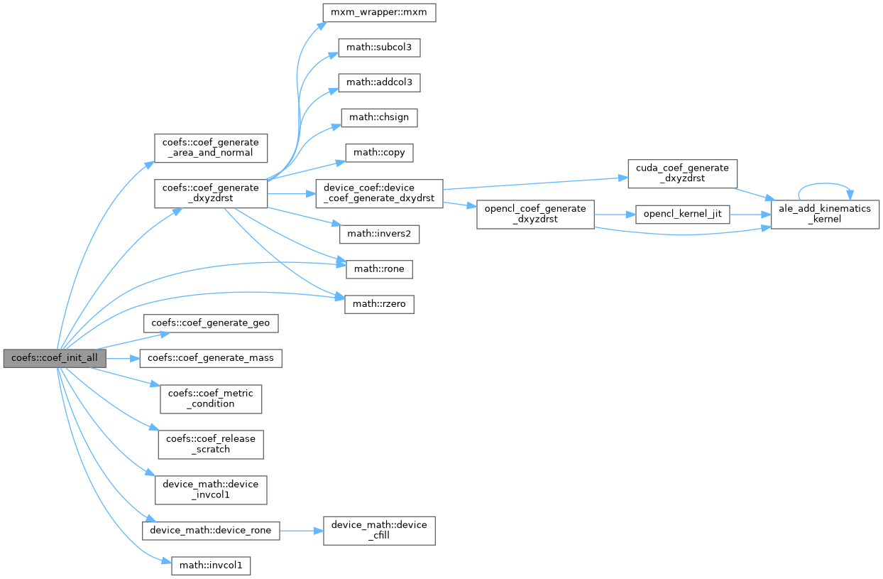
| subroutine | coef_init_all (this, gs_h, scope) |
| Initialize coefficients. | |
| subroutine | coef_free (this) |
| Deallocate coefficients. | |
| subroutine | coef_release_scratch (this) |
| Release the coefficients that COEF_OPERATOR does not retain. | |
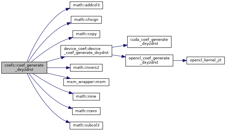
| subroutine | coef_generate_dxyzdrst (c) |
| subroutine | coef_generate_geo (c) |
| Generate geometric data for the given mesh. | |
| subroutine | coef_metric_condition (this) |
| Compute the metric tensor condition numbers over the mesh. | |
| subroutine | coef_enable_geo_compression (this, tol) |
| Enable compressed geometric factors. | |
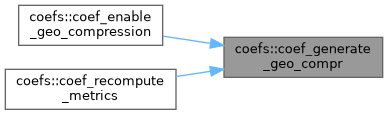
| subroutine | coef_generate_geo_compr (c, verbose) |
| Compute processor-local compressed versions of mappings Gij. | |
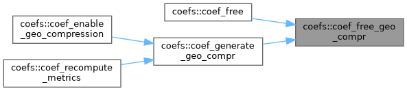
| subroutine | coef_free_geo_compr (c) |
| Release the compressed geometric factors. | |
| subroutine | coef_generate_mass (c) |
| Generate mass matrix B for the given mesh and space. | |
| subroutine | coef_require_facets (this, who) |
| Abort unless this coef holds the facet areas and normals. | |
| pure real(kind=rp) function, dimension(3) | coef_get_normal (this, i, j, k, e, facet) |
| Facet normal at a point. | |
| pure real(kind=rp) function | coef_get_area (this, i, j, k, e, facet) |
| Facet area at a point. | |
| subroutine | coef_generate_area_and_normal (coef) |
| Generate facet area and surface normals. | |
| subroutine | coef_generate_cyclic_bc (this) |
| subroutine | coef_recompute_metrics (this) |
| Recompute and update geometric factors (ALE) | |
| subroutine | coef_enable_lagged_mass (this) |
| Enable separate memory for lagged B matrices if needed. For eg. when mesh moves. | |
| subroutine | coef_update_lagged_mass (this) |
| Update history: Blaglag = Blag, Blag = B. | |
Variables | |
| real(kind=rp), parameter, public | neko_metric_cond_sp = 1.0e4_rp |
| Largest metric condition number for which single precision arithmetic on the geometric factors \( G_{ij} \) is considered safe, i.e. an rp = sp build. | |
| real(kind=rp), parameter, public | neko_metric_perturb_max = 1.0e-5_rp |
| Largest predicted relative perturbation of the element Helmholtz operator, in its own energy norm, for which single precision geometric factors are considered safe. | |
| integer, parameter, public | coef_full = 0 |
| Retain every coefficient. The default, and the only scope that supports recompute_metrics(), generate_cyclic_bc(), get_area(), get_normal() and any consumer of jac, jacinv, Binv or the derivative arrays. | |
| integer, parameter, public | coef_operator = 1 |
| Retain only what applying a discrete operator needs: \( G_{ij} \), h1, h2, B and mult. | |
Function/Subroutine Documentation
◆ coef_enable_geo_compression()
|
private |
Builds processor-local compressed copies of the geometric factors, see coef_generate_geo_compr(), for the operators that read them, e.g. ax_helm_compr_cpu_t, and rebuilds them with the geometry in recompute_metrics(). The copies are read by the CPU, SX and device backends, so nothing is built on the XSMM backend. Collective. Like the other diagnostics, the statistics are only logged under COEF_FULL, not for the operator-only coefficients of multigrid levels.
- Parameters
-
tol Tolerance on the difference of the geometric factors, summed over the element, under which two elements share them, defaults to 1e-7.
Definition at line 1577 of file coef.f90.

◆ coef_enable_lagged_mass()
◆ coef_free()

◆ coef_free_geo_compr()
|
private |
◆ coef_generate_area_and_normal()
|
private |

◆ coef_generate_cyclic_bc()
|
private |

◆ coef_generate_dxyzdrst()
|
private |

◆ coef_generate_geo()
|
private |

◆ coef_generate_geo_compr()
|
private |
Elements whose geometric factors agree share one copy of them in Gij_compr, and compression_inds maps each element to its copy. An element agrees with the first element of a copy when the absolute differences of their factors, summed over the quadrature points with the off-diagonal factors counted twice, are at most geo_compression_tol. Each element is compared with every copy found before it.
- Parameters
-
verbose Whether to log global statistics, which is collective.
- Note
- This could be faster with various tweaks
Definition at line 1621 of file coef.f90.

◆ coef_generate_mass()
|
private |

◆ coef_get_area()
|
private |
- Note
- Pure, see the note on coef_get_normal().
◆ coef_get_normal()
|
private |
- Note
- Pure, so it cannot reject a coef_t that lacks the normals. Consumers assert that themselves at setup, see coef_require_facets().
◆ coef_init_all()
|
private |
- Parameters
-
gs_h Gather-scatter handle carrying the dofmap to build on. scope Which coefficients to retain, COEF_FULL (default) or COEF_OPERATOR. See the scope parameters for what each one keeps.
- Todo:
- Be clever and try to avoid allocating zeroed geom. factors
Default values correspond to no rotation
Definition at line 376 of file coef.f90.
◆ coef_init_empty()
◆ coef_metric_condition()
|
private |
The stored geometric factors are \( G = w_3 J M \), where \( M \) is the metric matrix at a quadrature point. Both \( w_3 \) and the Jacobian are scalar multipliers, so \( \kappa(G) = \kappa(M) \) and the condition number of the stored \( G_{ij} \) is a pure property of the element geometry.
Two numbers are computed, because reduced precision arithmetic and reduced precision storage are limited by different properties of the element.
metric_cond is \( \kappa(G) \) and it governs the arithmetic. Applying \( D^T G D \) in precision \( \epsilon \) accumulates a quadratic form whose smallest eigendirection contributes a term of relative size \( 1/\kappa(G) \), which is lost once \( \kappa(G) \gtrsim 1/\epsilon \): about \( 1.7\times 10^{7} \) in single precision against \( 9\times 10^{15} \) in double. Below that the error grows as \( \epsilon\kappa(G) \); past it the local operator can turn indefinite and a Krylov solve breaks down rather than degrading. \( \kappa(G) \) grows as the square of the element aspect ratio, so a wall resolved boundary layer can approach the single precision limit while remaining ten orders clear of the double precision one. The single precision warning below is keyed on it.
metric_scaled_cond is \( \kappa(C) \) for the Jacobi scaled metric \( C_{ij} = G_{ij}/\sqrt{G_{ii}G_{jj}} \), the matrix of cosines between the contravariant basis vectors, and it governs storage. Rounding \( G_{ij} \) to a lower precision is a componentwise relative perturbation, so writing \( G = \Delta C \Delta \) with \( \Delta = \mathrm{diag}(\sqrt{G_{ii}}) \) the diagonal scaling passes through the rounding unchanged and cancels in every quadratic form. What remains bounds the relative perturbation of the element operator in its own energy norm by \( \epsilon\kappa(C) \), independent of the aspect ratio, of \( \kappa(G) \), of h and of the polynomial order: element stretching is invisible to storage rounding and only skew matters. Definiteness survives while \( \lambda_{min}(C) > 3\epsilon \), which in two dimensions means element edges more than about \( 0.02^\circ \) from parallel, so for storage this is a degenerate element test rather than an aspect ratio limit.
The two combine additively rather than as a pair of thresholds, because they are multiplied by different unit roundoffs – that of the precision \( G_{ij} \) is held in, and that of the precision the contraction accumulates in. metric_perturb reports \( \epsilon_{sp}\kappa(C) + \epsilon_{rp}\kappa(G) \), the predicted relative perturbation of the element operator were the factors held in single precision, and metric_sp_safe thresholds that against NEKO_METRIC_PERTURB_MAX. Gating on \( \kappa(G) \) alone is conservative by the square of the aspect ratio on a double precision build; gating on \( \kappa(C) \) alone would call an rp = sp build safe on a wall resolved mesh, which it is not.
- Note
- On device builds the host copy of \( G_{ij} \) is only refreshed at initialization, so this refreshes it itself when called later. It is not called from recompute_metrics(); a moving mesh that deforms significantly should invoke it explicitly.
Definition at line 1367 of file coef.f90.

◆ coef_recompute_metrics()
|
private |
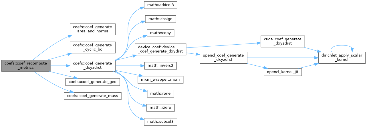
◆ coef_release_scratch()
The derivative arrays, the Jacobian and its inverse are scratch for \( G_{ij} \) and B, and are dead once those exist. Binv, the facet areas and the normals are never read when applying an operator. Called at the end of init; a no-op under COEF_FULL.
- Note
- area and the normals are not allocated at all under COEF_OPERATOR. They are listed here so the set of released coefficients is stated in one place.
Definition at line 857 of file coef.f90.

◆ coef_require_facets()
|
private |
For consumers of the facet metrics to call once at setup, so that being handed a COEF_OPERATOR coef fails at construction with a message naming the consumer, rather than dereferencing a released array mid solve. get_area() and get_normal() are pure and cannot report it themselves, and some consumers read nx, ny and nz directly and never go through them at all.
- Parameters
-
who Name of the consumer, used in the error message.
◆ coef_update_lagged_mass()
Variable Documentation
◆ coef_full
◆ coef_operator
The derivative arrays, jac and jacinv are scratch for \( G_{ij} \) and B, and Binv, area and the facet normals are never read by an operator, so all of them are released once the metrics are built. The work feeding only those is skipped as well: the facet metrics, the gather-scatter behind Binv, the volume reduction and the metric conditioning diagnostic.
Intended for multigrid levels, which read nothing else – see hsmg_init() and phmg_init(). The geometry cannot be rebuilt without the derivative arrays, so this scope is incompatible with a moving mesh.
◆ neko_metric_cond_sp
The hard limit is \( 1/\epsilon_{sp} \approx 1.7\times 10^{7} \), past which the smallest eigendirection of the metric is lost in the quadratic form and the element operator can lose positive definiteness. This keeps three orders of margin, which accepts isotropic, graded and channel interior meshes and rejects wall resolved ones; at the threshold itself the element operator already carries a relative error of order \( \epsilon_{sp}\kappa(G) \sim 10^{-3} \).
This threshold is about definiteness margin and is used only for the warning in coef_metric_condition(). Whether reduced precision is accurate enough on a given mesh is a separate question, answered by NEKO_METRIC_PERTURB_MAX and metric_sp_safe.
◆ neko_metric_perturb_max
The two metric condition numbers do not compete for a single threshold: they are multiplied by different unit roundoffs. Rounding \( G_{ij} \) for storage is a componentwise relative perturbation, and once the diagonal scaling in \( G = \Delta C \Delta \) cancels it contributes \( \epsilon_{store}\kappa(C) \) – element skew only. Accumulating \( D^T G D \) loses the smallest eigendirection of the metric and contributes \( \epsilon_{accum}\kappa(G) \) – aspect ratio squared. So the estimate is additive,
\[ \delta \approx \epsilon_{store}\kappa(C) + \epsilon_{accum}\kappa(G), \]
which needs no test on the build: an all double build is limited by neither term until \( \kappa(G) \sim 10^{13} \), a double build holding \( G_{ij} \) in single is limited by skew, and an rp = sp build is limited by aspect ratio, as it should be.
At \( 10^{-5} \) the storage term alone admits \( \kappa(C) \) up to about 84, i.e. element edges down to roughly \( 12^\circ \) apart, which is every mesh that is not close to degenerate. A well resolved double precision run whose discretisation error is smaller than this may want it tighter; coef_metric_condition() logs the estimate itself every run, so the value on a given mesh can be read rather than guessed, and reports when it is exceeded.
- Note
- The storage term is a genuine bound. The accumulation term is a bound up to a modest \( O(l_x) \) constant – measured about 4 at \( l_x = 6 \) – so leave margin.